
Acknowledgement
I would like to thank my supervisor, Dr Yongli Wang, for the constant support and guidance he has shown me throughout my dissertation. I would also like to thank Giulia, my friends and my family for supporting me throughout my time at the university.
1 Introduction
Bitcoin was the first cryptocurrency released in 2009 as open-source software, created by the pseudonymous Satoshi Nakamoto. Stock risk and return are generally calculated using the Sharpe ratio since its introduction (Sharpe, 1966; Sharpe, 1994). The Sharpe ratio will calculate the risk-adjusted returns to show the risk to reward of an asset in this case. The higher the ratio, the better reward to risk you will be achieving. While there have been numerous in-depth papers on cryptocurrencies in general, there is a limited number specifically on the risk and reward using the Sharpe Ratio and GARCH model (Chu et al. , 2017).
Many current literature pieces focus on Bitcoin specifically, but since 2014 Bitcoin’s market dominance as a percentage of total market capitalisation has slowly been falling from 95% in May 2013 to 40% as of May 2021, showing that alternative coins have become significantly more attractive to investors. Additionally, the ever-growing birth rate of cryptocurrencies will only decrease the dominance of Bitcoin. Therefore, the paper will look at many different cryptocurrencies that vary in market capitalisation which will add to the literature in this field.
The cryptocurrencies that will be used are Bitcoin (peer-to-peer digital currency), Ethereum (smart contract functionality), Binance coin (used in the Binance ecosystem), Dogecoin (meme coin), Litecoin (peer-to-peer digital currency), Monero (privacy-focused cryptocurrency, Dash (digital cash), DigiByte (peer-to-peer digital currency), Verge (privacy-focused cryptocurrency), BitShares (used in BitShares exchange ecosystem), Nexus (2 nd layer blockchain technology). The cryptocurrencies mentioned above vary in their use cases and this shows the diversity within the market.
The paper will be organised as follows: Section 2 will provide an overview of the literature, focusing on many different important aspects of cryptocurrencies. Section 3 will introduce the unit root test and GARCH models used in this study. Section 4 provides the detailed data description behind the model. Section 5 evaluates the findings of the model and the Sharpe Ratio. Section 6 concludes the findings of the paper and discusses its limitations of the paper.
2. Literature Review
Cryptocurrencies are built on decentralised networks using blockchain technology. The blockchain is a type of database that strings together the information from transactions made by a cryptocurrency. Furthermore, the blockchain is not controlled by one single person, it is controlled by all users. The information in the blockchain is irreversible and it is accessible to everyone. Bitcoin specifically gained mainstream attention in 2013 as a secure and cheaper way to send money. One way to measure the adoption of cryptocurrencies is to look at the market capitalisation change since its creation, which topped $2 trillion (Kharif, 2021). Alternatively, researchers have looked at the frequency of Google search keywords including cryptocurrencies (Bourgi, 2021). In light of the recent media attention that the cryptocurrency space has received, there have been a huge number of new projects dying and being created. Wu (2018) discovered that from 2015 to 2018 there was a significant increase in the birth and death rate of cryptocurrencies. From 2015 to 2018 there was more media attention than before and therefore more investors leading to an increase in the birth rate. As the birth rate increased, many new projects released did not have the backing or knowledge to flourish and therefore died, which resulted in a huge drawback for emerging projects. The drawback of projects was mainly seen at the end of the bull runs when the prices plummeted.
Chen et al (2016) examined through econometric analysis which ARCH model was best for the cryptocurrency index (CRIX). The authors discovered that a TGARCH (1,1) was the best-fitting model. However, when this model was used with my data set from August 2015 to June 2021 it was not the best fitting and therefore was not used. TGARCH is a threshold GARCH model which is mainly used when modelling asymmetric volatilities in financial data. Letra (2016), was creating a model which analysed the effects of daily Bitcoin prices on different search trends within Google and found that a GARCH (1,1) model was the best fit. Chu et al . (2017) found that after looking at model cryptocurrencies, the GARCH is the best fit when estimating value at risk.
Chuen et al (2018) examined the cryptocurrency index and the risk associated with investing in the index. The results show that incorporating the cryptocurrency index into a portfolio increases the Sharpe ratio, although they cautioned that the high ratios were not necessarily everlasting. Ahmed (2020) discovered significant evidence that shows that Bitcoin’s positive risk and return trade-off is unconfirmed. Rossi and Timmerman (2010) found that linear models cannot fully capture the relationship between volatility and returns. Barkai (2021) discovered that Bitcoin has the greatest risk-return portfolio, compared with Litecoin and Ripple, they lend this to the market dominance of Bitcoin.
2.1 Volatility
Jimoh and Benjamin (2020) discovered that in relation to bad news, the stock market reacts more volatile than the cryptocurrency market, however, this paper focused specifically on the Nigerian stock market which is significantly smaller than more developed markets such as the US stock market. Seys and Decaesteceker (2016) analysed the impact of news on the price of Bitcoin; they collected 22 events from 2015-2016. The authors discovered that rumours caused large price changes; however, this was only over a short period of time and with a small number of events, so a significant conclusion cannot be confirmed. The reason for most variation in price within cryptocurrencies comes from other projects innovating greater technologies and investors jumping from project to project (Lánský, 2016). Alternatively, Li and Wang (2017) believed that “the long-term Bitcoin exchange rate is more sensitive to economic fundamentals and less sensitive to technological factors”.
Caporale and Zekokh (2019) used a GARCH model to estimate and model the volatility within cryptocurrencies; they conclude that a considerable volume of users holds Bitcoin as a substitute for investing in the stock market. This is credited to the rapidly increasing cryptocurrency market.
Foley et al. (2019) stated: “Since cryptocurrency lacks intrinsic value, the exchange is shown to provide a pseudo-efficient trading platform for speculative investors.” This is reiterated by Nizzoli et al. (2020) who believed that cryptocurrencies are the market with the highest volume of financial speculation. This financial speculation is heavily correlated with cryptocurrencies’ abnormal volatility levels (Blau, 2017). The abnormal volatility and financial speculation lead to certain individuals achieving very quick returns on investments (Baur et al. , 2015). As investment opportunities, cryptocurrencies are very lucrative, however, the prices fluctuate too substantially for lending purposes.
Similarly, Foley et al. (2019), (Nizzoli et al. , 2020; Baur et al. , 2015; Cheah and Fry, 2015) stated that there are large cryptocurrency bubbles forming with significant financial speculation seen throughout cryptocurrency. Additionally, Grinberg (2011) found that the higher volatility specifically can lead to larger and more frequent speculative bubbles than traditional markets. The bubbles within the cryptocurrency market have been quite significant: in 2013, Bitcoin increased from $130 to just over $1,000 for it then burst and drop down to $200. These bursts have been quite considerable and have been repeating every couple of years as Corbet et al. (2017) have discovered.
Additionally, Baur et al. (2015) mentioned the increased ability for speculative attacks within cryptocurrencies as there is a lack of regulation like the stock market. This differs from Kristoufek (2014), who finds that the volatility within cryptocurrencies is caused predominantly by the investors’ interest. Several wealthy investment firms release statements or order huge selloffs to attempt to drive their price lower to buy them back significantly cheaper at a later stage. However, this is also seen in the stock market where hedge funds often order large selloffs to drive the price down. Catania and Grassi (2017) discovered that unlike exchange rates, the volatility dynamics in cryptocurrencies are significantly affected by leverages. Large leveraged positions can be liquidated very quickly, causing massive dips in the market. This differs from Ben and Xiaoqiong (2019), where the association between exchange rates and cryptocurrency performance is considerable.
The volatility in the cryptocurrency market has led to many firms reversing their stance on their acceptance of cryptocurrency as payment. This is because of the price difference from day to day, which causes financial forecasting to become very difficult for large global firms.
2.2 Comparison between how cryptocurrencies, fiat money and assets behave
To see how risk and return are linked within cryptocurrencies, it is important to try and distinguish what financial categories cryptocurrencies fall into. Initially, Nakamoto (2008) see Bitcoin as an alternative to traditional currencies and gold: this is also relayed by Li et al. (2020), who found that there were certain scenarios where Bitcoin behaves similarly to currencies and as a store of wealth. However, the authors mentioned that due to the uniqueness of the market, it may not behave in similar ways to other assets when exposed to a global event. This has partially been seen throughout the COVID-19 pandemic, where Bitcoin hit recent highs and oil crashed partway through the year.
While Bitcoin has been acknowledged as a commodity by the United States, Japan and El Salvador have declared it as a currency legally backed by the countries – does this constitute just Bitcoin being a fiat currency?
Fiat money has a few key characteristics – these include being backed by the government (centralised), having zero intrinsic value, being divisible, serving as a medium of exchange, store of value, and unit of account. In comparison, Bitcoin is currently being backed by El Salvadora as a legal tender, with a number of other smaller economies looking to adopt it. However, Tomić et al. (2020) stated that because the cryptocurrency market is regulated by private entities, the effect on the monetary system is significant. The authors stated that “Currently crypto does not have the capacity to endanger the international monetary system”. This could be potentially seen in a country of El Salvador’s economical stature which was ranked at a GDP of 103 out of 213 countries as seen in the world economic outlook database.
Bitcoin is decentralised and regulated by the network. It is durable and easily divisible. For Bitcoin to be a medium of exchange, cryptocurrencies still need to be more widely accepted but at the rate of acceptance that should not be too far into the future. One reason for the slow adoption of cryptocurrencies is the extremely high volatility which undermines the usage of Bitcoin as a medium of exchange and as a unit of account. Yermack (2015) assessed to see if Bitcoin is a real currency; they discovered that it fails to meet the criteria stated above, but that it has similar characteristics to speculative investment. Conversely, Bjerg (2016) found that Bitcoin is like “commodity money without gold, fiat money without a state”, which, from looking at the characteristics is accurate. Bitcoin and fiat money share many similarities, the key difference lies in whom it is controlled by. Governments can make the central banks print out more fiat money in contrast, most cryptocurrencies have a fixed supply and are controlled by private people or entities. Gervais et al. (2014) stated that Bitcoin is not a “normal” currency, it has lots of features from several different assets and currencies. One of those is the fact that it is much easier to store and is more secure than gold but does not have the stability that some individuals look for. Zimmerman et al. (2014) assessed individuals’ aims while using Bitcoin; they concluded that the users were predominately using it as an investment rather than as a method for transactions. This is due to the high volatility producing attractive easy and quick profits.
Dyhrberg (2016) explored the relationship between Bitcoin and virtual gold: they conclude that there are hedging capabilities. The main hedging capabilities are with the Financial Times Stock Exchange (FTSE) Index, Bitcoin can be used in conjunction with gold to minimise risk. Smith (2016) stated that Bitcoin is closer in the asset class to digital gold, but also discussed the correlation between currency exchange rates and Bitcoin price.
Wijk (2013) used the Dow Jones Index to show that Bitcoin is influenced by the stock market, but Kristoufek (2013) believed that this is because of the high speculation within the cryptocurrency market. Wang, Xue and Liu (2016) discovered that the oil prices and stock index do influence the price of Bitcoin in the short run, however in the long run there is a negative effect on Bitcoin’s price. Additionally, Ciaian, Rajacniova and Kancs, (2016), Bouoiyour and Selmi (2015) concluded that the variables such as oil prices do not impact the price of Bitcoin in the long term.
Many academic papers contradict each other, and in the cryptocurrency space, there has not been a clear consensus on the macroeconomic determinants that significantly affect the price of Bitcoin. This is mentioned by Vockathaler (2015), where results vary drastically when they are re-tested with new data. The author found that unexpected shocks such as power outages in China are the most significant factor in the volatility of Bitcoin. Likewise, Farell (2015) examined the key factors that affect growth and price and discovered that government regulation and retailers’ acceptance are significant.
Cryptocurrencies, and specifically the blockchain stop the double spending problem, as all transactions are checked and verified. However, with traditional banking, there can be errors where individuals will pay for the item twice. Making payments internationally can be cheaper and faster using cryptocurrencies as it is free to transfer any amount of TRX on the Tron Network within a few seconds. Internationally, it can cost upwards of 3-4% in fees and take up to 3 days. When a cash transaction takes place, both individuals need to be in the same location to exchange the money hence this creates difficulties in the case of long distances. Therefore, electronic payments were formed, and intermediaries and central authorities were created such as eBay. However, these intermediaries will take a small percentage as a handling fee.
Unlike credit card payments, transactions are irreversible; if someone steals your crypto information it is very unlikely you can get it back. Instead, with a credit card, you can cancel an order within 30 minutes, and it will be back in the bank account which is considerably more protection than cryptocurrencies. Additionally, within cryptocurrency, only the individual knows the address details, but with internet banking, you have the account number, sort code and full name of the individual. If fraud has taken place, it is easier to follow and retrieve. If you are banking within the United Kingdom with a regulated certified bank, the financial services compensation scheme (FSCS) will compensate an individual up to £75,000 if the bank goes out of business. This level of protection does not exist within cryptocurrencies.
2.3 Countries’ decisions on cryptocurrencies & regulation
Since Bitcoins’ creation, countries have been dealing with cryptocurrency regulation in three main ways: these are outright banning, a ‘wait and see approach’, and regulation. The different methods that countries use when making decisions vastly impact the price of cryptocurrencies and therefore the risk involved.
Banning consists of restricting the use of cryptocurrencies; this is either done by banning its acceptance as a currency or prohibiting banks and other companies from accepting deposits of cryptocurrencies. There are a few problems with this strategy, as individuals can use a VPN (a virtual private network) to change their online location to allow them to appear in a country that allows the buying and selling of cryptocurrencies. Furthermore, if a country bans cryptocurrency, then it cannot profit from the potential tax revenue and the advanced technology in place surrounding the market.
The ‘Wait and See Approach’ is used by governments who are unsure of the potential future or the threat that cryptocurrencies hold, and therefore do not see the need to regulate the market within the country. What has been seen in many countries is that governments have begun to issue warnings about the risks of investing in the cryptocurrency market. The warnings set by governments can dissuade individuals from investing and therefore reduce the volume and in turn the price.
Many cryptocurrency exchanges self-regulate to stay within the requirements of a country’s regulation or to try and provide greater protection for individuals against hackers. However, there is still an abundance of legal uncertainty and fraud risks, whether this is due to a lack of education on hacking and a basic understanding of the cryptocurrency world or regulation.
Plassaras (2013) suggest that cryptocurrencies should have a quasi-membership status within the IMF (international monetary fund) which would recognise cryptocurrencies and regulate them. There is still a lack of agreement on how to regulate cryptocurrencies across the world with many different countries taking alternative views. The European Union (EU) has taken the initiative by investing in many blockchain projects for the future (European Commission, 2020); this is the total opposite of China which has banned all cryptocurrencies and has stopped the process of mass cryptocurrency mining. After the investment by the EU, there has been a hesitancy about implementing too many regulations as they don’t want to hinder a growing market that they are a part of. Currently, the European Central Bank (ECB) does not consider virtual currencies as legal tender; however, there is a plan to create a digital Euro which will be a stablecoin (European Central Bank, 2021). Additionally, the US Federal Reserve has also indicated that they would like to digitise their currency to have a federally backed stablecoin. This is different from the United States of America Dollar Token (USDT), which is only partially backed by the US dollar and is in no way backed by the Federal Bank of America. These comments made by large governments lead individuals to become more confident that cryptocurrencies will be the future and thus increase the price.
To many investors, the appeal of cryptocurrencies is due to their unregulated nature and the fact that it is not controlled by an individual or government that can be corrupted. However, more regulation in the market could potentially lead to greater adoption of cryptocurrencies and allow them to be more freely available. Regulation could also increase stability, which would in turn lead it to share more characteristics with money.
3 Method
The main goal of the paper was to evaluate the relationship between risk and return within cryptocurrencies. In this case, the paper used the standardised volatility to capture the risk within an asset, as in most cases, the higher the volatility, the riskier the asset.
Figure 1 Bitcoin’s Residuals Plotted Versus Time
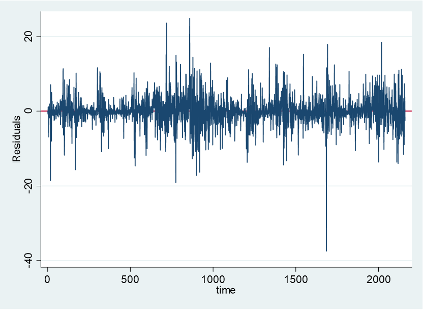
When looking at the residual chart in Figure 1 within Stata, there were several large clusters of data within the sample period chosen. Running an archlm test will demonstrate if there is an ARCH disturbance in the returns of Bitcoin. From this test, you can clearly see that the residuals are considerably distributed.
Using the Dicky-Fuller unit root test within the Bitcoin price there is non stationarity. With the rate of return using the Dicky-Fuller unit root test is significant at the 1% level and therefore there is stationarity in the variable.
The ARCH variance Model 1:
y t = σ t 2 = α 0 + α 1 e t − 1 2
Therefore, a variation of the ARCH model is needed to completely capture the effects.
y t is the variance at time t. α 0 is the conditional mean. α 1 is the volatility process. e 2 is the error term.
The ARMA-GARCH Model 2 general equation is as follows:
$$y_{t} = \ C + \ {\sum_{i = 1}^{m}{\phi_{i}y}}_{t - 1}\sum_{j = 1}^{n}{\theta_{j}\varepsilon_{t - j}} + \eta + \ \sum_{i = 1}^{p}{\beta_{i}\sigma_{t - i}^{2}}+\sum_{j = 1}^{q}{\alpha_{i}\varepsilon_{t - j}^{2}}$$
y t is the daily price of the specified financial item. C is a constant term. Ø i is the parameter of the autoregressive component of m. y t-1 is the lagged daily price of the specified financial item. θ j is the parameter of the moving average component of n. ε t-j is the error term. η is the long run volatility. β is how often volatility is present and α is how new information affects volatility. Which is also seen in Ghani and Rahim (2019).
This is an ARMA(m,n) and GARCH(p,q) model. From a range of different models, one model was selected by using the Bayesian (1978) information criterion (BIC) and the Akaike (1974) information criterion (AIC). The BIC and AIC are used in the selection of multiple fitting models. The BIC initially was created by Gideon Schwarz in 1978 but was developed by Bayesian; AIC was developed by Hirotsugu Akaike in 1973. The main difference between the two models selecting criteria is the harsher penalty in BIC for more parameters. The BIC and AIC help to identify the lags needed in ARMA-GARCH models. Using both information criteria a GARCH (1,1) was selected. This selection is in-line with most literature findings seen in the literature review. The GARCH (1,1) model was then used to calculate residual diagnostic checks to see if there was sufficient white noise in the model. The ARMA part of the equation m and n is zero as suggested by the BIC. The GARCH (Bollerslev, 1986) model adds lags to the variance, Model 3 is shown below and is defined in Bollerslev’s paper:
h
1
=
δ
+
α
1
e
t
− 1
2
+
β
1
h
t
− 1
To use the estimated standardised volatility calculated above, Ahmed’s (2020) model will be slightly altered through a range of regressions in order to view the return to risk of Bitcoin and other cryptocurrencies. This regression will be an Ordinary Least Squares (OLS) regression with robust standard errors. To deal with the potential endogeneity in the model there will be a generalized methods of moments (GMM) approach.
The Sharpe Ratio:
SR = $$\frac{R_{p} + R_{f}}{\sigma_{p}}$$
Where R p is the return of the portfolio specified. R f is the risk-free rate calculated using the risk-free rate specified by the US government. σ p is the standard deviation of the portfolio’s excess return.
The Sharpe ratio will be calculated to allow the bilateral comparison between the different assets shown. The Sharpe ratio adjusts a portfolio expected for risk and concludes how much excess return will be received for an additional unit of risk. Sharpe (1994) states that the Sharpe ratio may not give a reliable portfolio ranking if assets are correlated. Therefore, each asset will be in its own portfolio to not affect other assets negatively or positively as the correlations to Bitcoin can be seen in Table 1.
Ahmed (2020) model:
$$R_{t} = \ \alpha + \ \sum_{i = 1}^{q}{R_{t - i} + \ \beta V_{t - 1} + \ \varepsilon_{t}}$$
Where R t is the return of Bitcoin. α is the intercept. R t-i is the return of Bitcoin lagged by one period. V t-1 is the volatility lagged by one time period. ε t is the error term.
After altering the model by Ahmed (2020) of Risk-Return shown above, regression 1 below was formed.
Model in Regression 1:
B
R
t
=
β
1
+
β
2
B
R
t
− 1
+
β
3
V
t
+
ϵ
t
Where BR t is Bitcoin’s daily return at time t. β 1 is the intercept term. β 2 is the constant attached to B R t − 1 which is Bitcoin’s daily return at one previous time period. β 3 is the constant attached to V t which is the volatility of Bitcoin at time t. ϵ t is the stochastic disturbance term within the model. When β 2 is positive and significant, it will indicate that a higher previous time return rate will increase the current return rate of Bitcoin. When β 3 is positive and significant, it will imply that higher volatility stimulates higher returns. This would explain a presence of a risk-return trade-off, the volatility may be lagged in future regressions to see if there is a time variance between the returns and volatility. The volatility calculated in this model is estimated using the GARCH (1,1) model previously shown. The GARCH (1,1) model was the best fitting to the data series.
The 2 nd regression:
B
R
t
=
β
1
+
β
2
B
R
t
− 1
+
β
3
V
t
+
β
4
L
B
T
C
P
+
ϵ
t
Where the variables are the same as regression 1, however, LBTCP is the log of Bitcoins price. This variable was added to the regression as it shows the returns and how those changes as the logged price increases.
The 3 rd regression:
B
R
t
=
β
2
B
R
t
− 1
+
β
3
V
t
+
ϵ
t
Where the variables are the same as regression 1, however, the constant has been removed. The constant was removed as it was not significant in the previous two models. However, without the constant the model is forced through (0,0).
The 4 th regression:
B
R
t
=
β
2
B
R
t
− 1
+
β
3
V
t
+
β
4
V
t
− 1
+
ϵ
t
There is not a constant which is also seen in the 3 rd regression, additionally, a lagged volatility term subscript has V t − 1 has been added which is seen in Ahmed’s (2020) paper.
The 5 th regression:
B
R
t
=
β
3
V
t
+
ϵ
t
Where β 1 + β 2 B R t − 1 has been removed from model 1, which is the constant and the Bitcoin returns lagged by one time period, being a singular day.
LBTC
R
t
=
β
1
+
β
2
B
R
t
− 1
+
β
3
V
t
− 1
+
ϵ
t
Where LBTCR t is logged Bitcoin return at time t and V t-1 is the volatility lagged by one period of time and the rest of the equation is the same as the model stated in regression 1. This is to see the difference in results and significance when the returns are logged.
4 Data
The daily data of cryptocurrencies are taken from the Coinmarketcap (which is a website that has daily data points for cryptocurrencies) and range from August 2015- June 2021, except for Binance coin, which was created in 2017. The market capitalisations are taken from the 23 rd of July 2021. The other assets (Oil, Gold, S&P, US Dollar) were taken from uk.investing and all range from August 2015- June 2021.
Listed below are 12 cryptocurrencies with varying market capitalisation, to see if there is a variation in the Sharpe ratio due to market capitalisation. When deciding which cryptocurrencies to use, this dissertation used the oldest cryptocurrency in each specific market capitalisation to ensure that there were many data points, to guarantee accuracy. This also ensures that the time series is not affected differently through bull and bear runs. Using the time period from August 2015 – June 2021 will provide a large sample (roughly 2159 data points), showing 2 distinctive bull runs (2018, 2021) and a less distinctive bull run in (mid-2019). BNB (Binance coin) has been added from July 2017 as such a large cryptocurrency with only Tether close in market capitalisation. Tether (USDT) cannot be included as it is pinned to the US dollar. The cryptocurrency abbreviations are as followed: Bitcoin (BTC), Ethereum (ETH), Binance Coin (BNB), Dogecoin (DOGE), Litecoin (LTC), Monero (XMR), Dash (DASH), DigiByte (DGB), Verge (XVG), Bitshares (BTS), Syscoin (SYS), Nexus (NXS).
The Risk-free rate of government bonds in the United States of America is 2% according to the United States government website which was used when calculating the Sharpe ratio. The other traditional assets include S&P (Standard and Poor) 500, Oil, US Dollar Index and Gold. These assets have a daily date range from August 2015- June 2021. There are fewer data points with traditional assets as the trading markets are closed on weekends and bank holidays.
Table 1 A detailed table of different cryptocurrency assets and a comparison to more traditional assets
| Asset | Market Cap in USD $ | Sharpe Ratio | % Returns >0 | Mean | SD | T Statistic | Correlation to BTC returns |
|---|---|---|---|---|---|---|---|
| BTC | 636,359,806,389 | 1.6 | 55.14 | 0.30% | 3.98% | 3.55 | 1 |
| ETH | 253,556,810,462 | 1.64 | 50.81 | 0.53% | 6.50% | 3.81 | 0.02686 |
| BNB* | 51,043,467,728 | 4.11 | 52.15 | 0.85% | 8.02% | 4.01 | -0.0539 |
| DOGE | 25,480,262,751 | 1.14 | 48.58 | 0.69% | 10.80% | 2.98 | 0.3344 |
| LTC | 8,418,391,849 | 0.71 | 49.57 | 0.33% | 5.81% | 2.61 | 0.6498 |
| XMR | 3,735,691,095 | 1.32 | 51.02 | 0.49% | 6.64% | 3.40 | 0.5331 |
| DASH | 1,481,991,314 | 0.70 | 49.46 | 0.36% | 6.25% | 2.66 | 0.5183 |
| DGB | 581,783,863 | 0.93 | 47.54 | 0.76% | 10.94% | 3.25 | 0.3549 |
| XVG | 319,194,713 | 0.79 | 49.51 | 1.25% | 14.70% | 3.92 | 0.2809 |
| BTS | 120,488,172 | 0.27 | 48.14 | 0.41% | 8.26% | 2.31 | 0.4321 |
| SYS | 78,494,933 | 0.77 | 50.08 | 0.67% | 9.62% | 3.24 | 0.3630 |
| NXS | 33,008,960 | 0.81 | 50.70 | 0.77% | 10.43% | 3.42 | 0.3391 |
| Average for cryptocurrencies | / | 1.23 | 50.23 | 0.62 % | 8.50% | 3.26 | 0.3435 |
| Traditional Assets | |||||||
| Oil | / | (0.20) | 45.95 | 0.01% | 2.73% | 0.13 | -0.0065 |
| Gold | / | 0.47 | 52.79 | 0.04% | 0.86% | 1.61 | -0.0093 |
| S&P | / | 0.57 | 55.08 | 0.06% | 1.19% | 1.80 | -0.201 |
| US Dollar Index | / | (0.48) | 52.13 | -0.003% | 0.38% | -0.30 | -0.0196 |
* BNB from 26 th July 2017
The difference in the standard deviation between the two is significant; specifically, gold and the cryptocurrency average are 0.86% and 8.50% respectively. This vast difference shows the increased volatility within the market. Surprisingly, the number of days that have positive returns while holding Bitcoin is 55.14%, which is significantly higher when compared to the cryptocurrency average. However, when compared to traditional assets such as the S&P, it is much more in line with expectations. There does not seem to be a trend between market capitalisation and the Sharpe ratio. Conversely, as expected, the volatility within smaller market capitalisation cryptocurrencies was greater than the larger market capitalisation cryptocurrencies (Wang et al. , 2019). The negative Sharpe ratio seen in oil and the US Dollar Index is due to the risk-free rate being larger than the returns of the asset. The T statistic is a test to see whether the returns of that specific cryptocurrency are larger than zero.
Wang et al. (2019) found that small market value cryptocurrencies have higher average returns. In the data that is observed above, the smaller market capitalisation cryptocurrencies have larger than average mean returns, which is in line with the findings from Wang et al. (2019).
When deciding whether to invest into a certain portfolio, the Sharpe ratio is often calculated. If a portfolio has a ratio of 0.2-0.5 then it is acceptable and is in line with the market expectations. An above average Sharpe ratio is 0.5-1. Anything greater than 1 is viewed as good by investors, half of the 12 cryptocurrencies have a Sharpe ratio of over 1. This shows that although there is a large increase in the risk and volatility within the cryptocurrency market, the rewards are worth the risk. While the more traditional assets only outperformed one cryptocurrency in the sample, Binance coin has the highest Sharpe ratio calculated at 4.11, which is more than likely due to the shorter time period recorded.
Most of the alternative assets are close enough to zero to have no correlation apart from the S&P which is -0.201; this correlation is most likely too small to be significant. However, the correlation between Bitcoin and Litecoin (0.6498) is significantly positive which was expected due to a large number of similarities in functions. Looking at the average cryptocurrency correlation to Bitcoin, there is a weak positive correlation. Oil has little to no effect on Bitcoin and the correlation is insignificant which is seen in Ciaian, Rajacniova and Kancs (2016), and Bouoiyour and Selmi (2015).
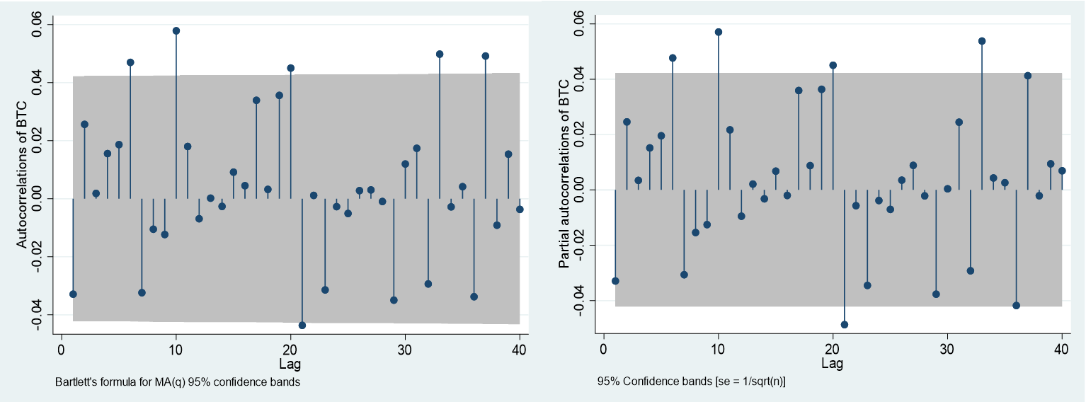
The correlogram tool is useful when using empirical time series data; these show the similarity between BTC and the lagged versions of Bitcoin over several time periods. Figure 2 below shows that there is autocorrelation, but through tests within Stata, they are not significant enough. Additionally, there does not seem to be a pattern when looking at the colleogram graph showing that the points are more than likely random. The colleograms in Figure 2 shows that there is stationarity within the series as the time does not have a visual trend. Additionally, using the Dicky-fuller unit root test on Bitcoin returns shows that the returns were stationary within the series.
Figure 2 Autocorrelation and Partial Correlation Within Bitcoins Returns
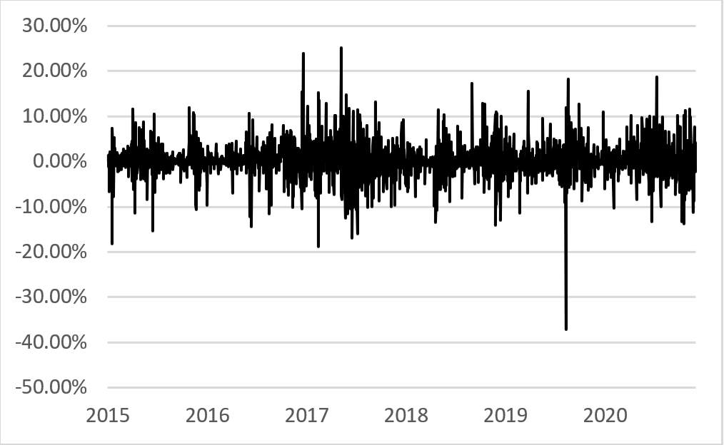
Figures 3 and 4 shown below explain the historical levels of Bitcoin and the Returns of Bitcoin over the sample period. The price of Bitcoin as seen over the sample period indicates two distinctive bull markets (where the financial asset in this case Bitcoin is increasing over time) and a smaller peak in 2019. The daily returns of Bitcoin in a percentage form can be seen that indicates the extreme levels of volatility throughout the sample period. The sharp decline towards the end of 2019 can be attributed to the speculation of Bitcoin halving which happened in 2020.
Figure 3 Bitcoins’ Price Level in USD ($) Over the Periods 2015-2021
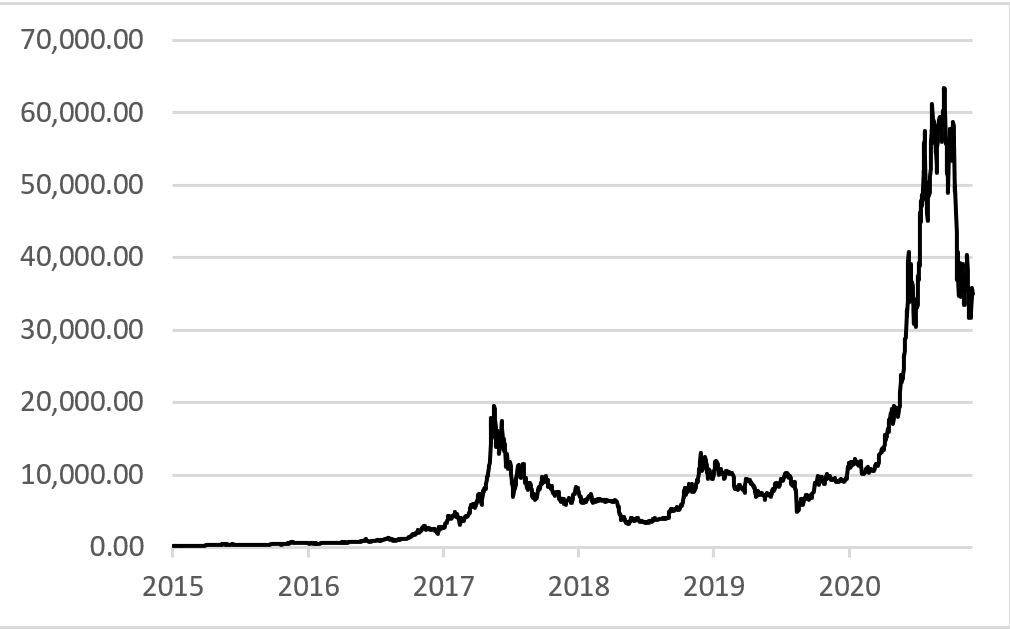
Figure 4 Bitcoin Returns (%) Over the Periods 2015-2021
5 Empirical results
Below in Table 2, the estimations for the other 11 cryptocurrencies were completed using a GARCH (1,1) model as this is what was selected when using the AIC and BIC information criteria for each cryptocurrency data. Below only the returns compared to the volatility of the specified cryptocurrency are shown with no constant which is regression 5. The volatility in the tests is the volatility of the specified cryptocurrency, not Bitcoins. These tests are done with robust standard errors. V is the volatility coefficient. Additionally, the volatility of the traditional asset is shown below, however, a GARCH (1,1) was used.
| ETH | BNB | DOGE | LTC | XMR | DASH | DBG | XVG | BTS | SYS | NXS | Gold | S&P | Oil | USD | |
|---|---|---|---|---|---|---|---|---|---|---|---|---|---|---|---|
| V | 0.12*** | 0.18*** | 0.07*** | 0.07*** | 0.08*** | 0.06** | 0.08*** | 0.13*** | 0.04 | 0.06** | 0.07** | 0.04 | 0.04 | 0.07* | 0.002 |
| (0.03) | (0.05) | (0.03) | (0.04) | (0.03) | (0.03) | (0.03) | (0.04) | (0.03) | (0.03) | (0.03) | (0.03) | (0.08) | (0.05) | (0.03) | |
| N | 2154 | 1436 | 2160 | 2160 | 2160 | 2160 | 2160 | 2160 | 2160 | 2160 | 2160 | 1539 | 1488 | 1525 | 1543 |
|
|||||||||||||||
|
|||||||||||||||
|
Table 2 Standardised volatility measures using a GARCH (1,1) model
These results are almost all significant at the 1% level for the cryptocurrencies, and the results show that there is not a larger difference in volatility when the market capitalisation changes with the largest to smallest capitalisation ranging from left to right. Additionally, as the rate of return increases by 10% the Ethereum volatility will increase by 119%. Instead, when oil’s rate of return increases by 10%, the volatility only increases by 75% which is slightly lower than five out of the twelve cryptocurrencies shown. The table of traditional assets is not very significant probably due to the GARCH (1,1) model used because it is tailored for Bitcoin specifically, and therefore it will not necessarily translate very well to other asset classes.
Table 3 Regression from the models shown above
| Dependent Variable: BTCROI | Dependent Variable: LogBTCROI | |||||
|---|---|---|---|---|---|---|
| Independent Variable | (1) | (2) | (3) | (4) | (5) | (6) |
| β 1 | 0.000264 | 0.005432 | -5.373804*** | |||
| (0.002762) | (0.004601) | (0.101991) | ||||
| lagBTC1 | -0.033293 | -0.033104 | -0.033260 | -0.030420 | -1.187217 | |
| (0.032478) | (0.032406) | (0.021513) | (0.021490) | (0.896941) | ||
| Volatility | 0.074420 | 0.094816 | 0.083897*** | 0.599673*** | 0.077940*** | |
| (0.078976) | (0.060429) | (0.020769) | (0.174859) | (0.025581) | ||
| logBTCPrice | -0.000720 | |||||
| (0.006135) | ||||||
| LagVolatility1 | -0.523225*** | 28.569478*** | ||||
| (0.174946) | (2.505672) | |||||
| N | 2159 | 2159 | 2159 | 2159 | 2160 | 1189 |
| R 2 | 0.0018 | 0.0025 | 0.0076 | 0.0117 | 0.065 | 0.1012 |
| R 2 Adj | 0.0009 | 0.0011 | 0.0067 | 0.0103 | 0.067 | 0.0997 |
| DW | 1.996 | 1.9968 | 1.9968 | 1.9932 | 1.993 | 0.9228 |
Robust standard errors in parentheses
***= 1% significance level
**= 5% significance level
*= 10% significance level
The 1 st regression does not yield any significant variables at any level, therefore, the model used in regression one will need to be altered.
The 2 nd regression the log of Bitcoins price has been added and this again does not yield any significant variables. However, as seen in regression 1, the volatility measures are similar values to some of the literature researched.
In the 3 rd regression, the constant β 1 is removed from the model, volatility is now significant at the 1% level. The significant volatility measure shows that as Bitcoin returns increase by 10% the volatility also increases by 83%, which can be seen when looking at the volatility bands within exchange sites.
Regression 4 provides interesting results with significant volatility measures for the present period and lagged period, where the volatility increase (risk) causes a large increase in the rate of return of Bitcoin. Additionally, both lagged terms (returns and volatility) have negative coefficients, however, the lagged rate of return of Bitcoin is not significant.
The 5 th regression examines Bitcoins returns directly onto the volatility, and as returns increase by 10% the volatility also increases by 77.9%. The volatility here is significant at the 1% level and provides a useful insight into the risk-return of Bitcoin.
The 6th regression uses the log of Bitcoins’ daily returns as the dependent variable which differs from the other regressions. The lagged volatility is significant and positive which shows that as the volatility increases so does the log of Bitcoins returns, which indicates that there is a risk-return reward. However, as some of the rates of returns are too close to zero in size then many logged variables are zero, which reduces the number of observations. The reduction in certain observations has altered the Durbin-Watson test from around 2 for regressions 1-5 to 0.92 in regression 6 showing some positive autocorrelation.
6 Conclusion
To conclude, cryptocurrency returns are significantly higher than more traditional methods, whether you use the Sharpe ratio or look at the standardised volatility using GARCH modelling. There is a significant increase in risk, but also considerable returns that outweigh the present risk. Using the estimations calculated above cryptocurrencies are roughly 7x riskier than the S&P 500 index as well as having a mean which is around 10x larger. The cryptocurrency market having such high levels of returns is not sustainable for itself or any other tradable asset market. While looking at the Sharpe ratio, widely used in risk-return forecasting, cryptocurrencies have on average almost twice as large of a Sharpe ratio. If investors are going to invest within the cryptocurrency market, then a diversified portfolio with an increased number of larger capitalisation coins would yield the highest Sharpe ratio. This is seen in Brauneis and Mestel (2019) who find that there is a significant reduction in risk when there is a portfolio containing many different cryptocurrencies. This allows for investors who are risk averse to still benefit from cryptocurrencies without the abnormal single portfolio risk rates.
6.1 Limitations
A large limitation is that the current bull run has not ended yet so data cannot be calculated, so to have data once this bull run has ended would help to have distinctive bull runs to view and breakdown, along with more research to view the returns within a bull run. Additionally, there are lots of current regulations being discussed by different governments leading to a lot of scepticism, which may have an impact on the volatility and returns. In the future, a more detailed look into other more complex models would potentially allow for a better fitting and more accurate model which would be able to further estimate volatility or mean returns.
References
Ahmed, W.M., 2020. Is there a risk-return trade-off in cryptocurrency markets? The case of Bitcoin. Journal of Economics and Business , 108 , p.105886.
Barkai, I., Shushi, T. and Yosef, R., 2021. A Cryptocurrency Risk–Return Analysis for Bull and Bear Regimes. The Journal of Alternative Investments .
Baur, A.W., Bühler, J., Bick, M. and Bonorden, C.S., 2015, October. Cryptocurrencies as a disruption? empirical findings on user adoption and future potential of bitcoin and co. In Conference on e-Business, e-Services and e-Society (pp. 63-80). Springer, Cham.
Ben, S. and Xiaoqiong, W., 2019. Are Cryptocurrencies Good Investments?. Studies in Business & Economics , 14 (2).
Bjerg, O., 2016. How is bitcoin money? Theory, Culture & Society , 33 (1), pp.53-72.
Blau, B.M., 2017. Price dynamics and speculative trading in bitcoin. Research in International Business and Finance , 41 , pp.493-499.
Bollerslev, T., 1986. Generalized autoregressive conditional heteroskedasticity. Journal of Econometrics , 31 (3), pp.307-327.
Bouoiyour, J. and Selmi, R., 2015. What does Bitcoin look like?. Annals of Economics & Finance , 16 (2).
Bourgi, S (2021) ‘Buy Crypto’ Google search hit record high: The Tie, available at: https://cointelegraph.com/news/buy-crypto-google-searches-hit-record-high-the-tie (accessed 14th of July 2021)
Brauneis, A. and Mestel, R., 2019. Cryptocurrency-portfolios in a mean-variance framework. Finance Research Letters , 28 , pp.259-264
Caporale, G.M. and Zekokh, T., 2019. Modelling volatility of cryptocurrencies using Markov-Switching GARCH models. Research in International Business and Finance , 48 , pp.143-155.
Catania, L. and Grassi, S., 2017. Modelling crypto-currencies financial time-series. Available at SSRN 3028486 .
Cheah, E.T. and Fry, J., 2015. Speculative bubbles in Bitcoin markets? An empirical investigation into the fundamental value of Bitcoin. Economics letters , 130 , pp.32-36.
Chen, S., Chen, C., Härdle, W.K., Lee, T.M. and Ong, B., 2016. A first econometric analysis of the CRIX family. Available at SSRN 2832099 .
Chu, J., Chan, S., Nadarajah, S. and Osterrieder, J., 2017. GARCH modelling of cryptocurrencies.
Journal of Risk and Financial Management
,
10
(4), p.17.
Ciaian, P., Rajcaniova, M. and Kancs, D.A., 2016. The economics of BitCoin price formation.
Applied Economics
,
48
(19), pp.1799-1815.
Coinmarketcap, https://coinmarketcap.com/ – Data for the 12 Cryptocurrencies (accessed on the 23 rd of July 2021)
Corbet, S., Lucey, B. and Yarovaya, L., 2018. Datestamping the Bitcoin and Ethereum bubbles. Finance Research Letters , 26 , pp.81-88.
Chuen, D.L.K., Guo, L. and Wang, Y., 2017. Cryptocurrency: A new investment opportunity?. The Journal of Alternative Investments , 20 (3), pp.16-40.
Dyhrberg, A.H., 2016. Hedging capabilities of bitcoin. Is it the virtual gold?. Finance Research Letters , 16 , pp.139-144.
Engle, R.F., 1982. Autoregressive conditional heteroscedasticity with estimates of the variance of United Kingdom inflation. Econometrica: Journal of the econometric society , pp.987-1007.
European Commission (2021) Blockchain funding and investment, available at: https://digital-strategy.ec.europa.eu/en/policies/blockchain-funding (accessed 13th July 2021)
European Central Bank (2020) A digital euro, available at: https://www.ecb.europa.eu/paym/digital_euro/html/index.en.html (accessed 13th July 2021)
Farell, R., 2015. An analysis of the cryptocurrency industry.
digital currencies: bringing Bitcoin within the reach of IMF. Chi. J. Int'l L. , 14 , p.377.
Florea, I.O. and Nitu, M., 2020. Money Laundering Through Cryptocurrencies. Romanian Economic Journal , 22 (76), pp.66-71.
Foley, Karlsen, Putnins (2019) “Sex, Drugs and Bitcoin: How much illegal activity is financed through cryptocurrencies” The review of Financial studies v32 p1798-1853 https://academic.oup.com/rfs/article/32/5/1798/5427781
Gervais. A, Karame. G, Capkun. V, Capkun. S (2014) “Is Bitcoin a Decentralized Currency?” ISEE Security & Privacy V12 i3 p54-60 https://doi.org/10.1109/MSP.2014.49
M Md Ghani and H A Rahim 2019 IOP Conf. Ser.: Mater. Sci. Eng. 548 012023
Heaven, W. (2018) Sitting with the cyber-sleuths who track cryptocurrency criminals, Available at: https://www.technologyreview.com/2018/04/19/3011/sitting-with-the-cyber-sleuths-who-track-cryptocurrency-criminals/ (accessed 25 th of July 2021)
ISEE Security & Privacy V12 i3 p54-60 https://doi.org/10.1109/MSP.2014.49
Jimoh, S.O. and Benjamin, O.O., 2020. The Effect of Cryptocurrency Returns Volatility on Stock Prices and Exchange Rate Returns Volatility in Nigeria. Acta Universitatis Danubius. Œconomica , 16 (3).
Kharif, O. (2021) Crypto Market Cap Surpasses $2 Trillion After Doubling This Year, available at: https://www.bloomberg.com/news/articles/2021-04-05/crypto-market-cap-doubles-past-2-trillion-after-two-month-surge (accessed 14th of July 2021)
Kristoufek, Ladislav (2013). “BitCoin meets Google Trends and Wikipedia: Quantifying the relationship between phenomena of the Internet era”. In: Scientific reports 3, p. 3415.
Kristoufek, L., 2014. What are the mai price? Evidence from wave analysis.
Lánský, J., 2016. Analysis of cryptocurrencies price development. Acta Informatica Pragensia , 5 (2), pp.118-137.
Letra, I.J.S., 2016. What drives cryptocurrency value? A volatility and predictability analysis (Doctoral dissertation, Instituto Superior de Economia e Gestão).
Li, X. and Wang, C.A., 2017. The technology and economic determinants of cryptocurrency exchange rates: The case of Bitcoin. Decision support systems , 95 , pp.49-60.
Li, Y., Zhang, W., Xiong, X. and Wang, P., 2020. Does size matter in the cryptocurrency market?. Applied Economics Letters , 27 (14), pp.1141-1149.
Nakamoto, S., 2008. Bitcoin: A peer-to-peer electronic cash system. Decentralized Business Review , p.21260.
Nizzoli, L., Tardelli, S., Avvenuti, M., Cresci, S., Tesconi, M. and Ferrara, E., 2020. Charting the landscape of online cryptocurrency manipulation. IEEE Access , 8 , pp.113230-113245.
Rossi, A.G. and Timmermann, A., 2010, March. What is the shape of the risk-return relation?. In AFA 2010 Atlanta Meetings Paper .
Seys, J. and Decaestecker, K., 2016. The evolution of Bitcoin price drivers: Moving towards stability. Unpublished Masters’ Thesis. University of Ghent, Gent .
Sharpe, W.F., 1994. The Sharpe ratio. Journal of portfolio management , 21 (1), pp.49-58.
Smith, H.J., 2016. Technical analysis of the Bitcoin cryptocurrency (Doctoral dissertation, Hochschule für angewandte Wissenschaften Hamburg).
Tomić, N., Todorović, V. and Čakajac, B., 2020. The potential effects of cryptocurrencies on monetary policy. The European Journal of Applied Economics , 17 (1), pp.37-48.
Uk.investing https://uk.investing.com/commodities/gold - Data from Gold, Oil, USD, S&P (accessed on the 23 rd of July 2021)
Van Wijk, D., 2013. What can be expected from the BitCoin? Erasmus Universiteit Rotterdam , 18 .
Vockathaler, B., 2015. The bitcoin boom: An in depth analysis of the price of bitcoins.
Wang, J., Xue, Y. and Liu, M., 2016, July. An analysis of bitcoin price based on the VEC model. In Proceedings of the 2016 International Conference on Economics and Management Innovations .
World economic outlook database, 2021 International Monetary Fund, IMF.org (accessed on 27 th of august 2021) https://www.imf.org/en/Publications/WEO/weo-database/2021/April/weo-report?c=512,914,612,614,311,213,911,314,193,122,912,313,419,513,316,913,124,339,638,514,218,963,616,223,516,918,748,618,624,522,622,156,626,628,228,924,233,632,636,634,238,662,960,423,935,128,611,321,243,248,469,253,642,643,939,734,644,819,172,132,646,648,915,134,652,174,328,258,656,654,336,263,268,532,944,176,534,536,429,433,178,436,136,343,158,439,916,664,826,542,967,443,917,544,941,446,666,668,672,946,137,546,674,676,548,556,678,181,867,682,684,273,868,921,948,943,686,688,518,728,836,558,138,196,278,692,694,962,142,449,564,565,283,853,288,293,566,964,182,359,453,968,922,714,862,135,716,456,722,942,718,724,576,936,961,813,726,199,733,184,524,361,362,364,732,366,144,146,463,528,923,738,578,537,742,866,369,744,186,925,869,746,926,466,112,111,298,927,846,299,582,487,474,754,698,&s=NGDPD,&sy=2021&ey=2021&ssm=0&scsm=1&scc=0&ssd=1&ssc=0&sic=0&sort=country&ds=.&br=1
Wu, K., Wheatley, S. and Sornette, D., 2018. Classification of cryptocurrency coins and tokens by the dynamics of their market capitalizations. Royal Society open science , 5 (9), p.180381.
Yermack, D., 2015. Is Bitcoin a real currency? An economic appraisal. In Handbook of digital currency (pp. 31-43). Academic Press.
©Harvey Grew. This article is licensed under a Creative Commons Attribution 4.0 International Licence (CC BY).